


Abstract
There is an increasing resource assessment and management requirement for single-tree-based stand models due to a shift towards mixed-species and ‘back to nature’ forestry. This paper describes the validation and calibration of the CARBWARE stand simulator, a distance-independent single-tree growth modelling framework specifically modified to include spatially explicit climatic and soil factors. Tree growth functional analysis suggests that stand competition factors contribute to most (21–33 per cent) of the observed variation in diameter increment, followed by tree size factors (17–20 per cent). Edaphic and other site factors, particularly soil nutrition and moisture status, explained 4–11 per cent of the observed site-to-site variation. The developed empirical relationships may provide a deterministic framework for improving developed ecological site classification systems. Independent validation showed that the CARBWARE simulator provides a robust and un-bias estimate of single-tree and stand-based variables for both pure and intimate mixed stands. However, refinements to the simulator are still required, particularly improvement to climatic and genetic response factors, mortality functions for mixed-species stands and inclusion of regeneration/recruitment models.
Introduction
Single-tree growth models simulate changes in forest stand dynamics as a mosaic of individual trees with or without consideration of positional dependence within the stand (Hasenauer, 2006; Pretzsch, 2009). Although single-tree-based stand models were initially developed for even-aged and pure stands (Newnham, 1964; Mitchell, 1975), application to mixed-species and uneven-aged stands (Wykoff, 1990; Monserud and Sterba, 1996) has proven to be valuable, particularly for application under ‘back to nature’, mixed-aged forests and continuous cover forestry management scenarios (Hasenauer, 2006). Given the change in silvicultural management objectives towards more mixed-species and uneven-aged forests in Europe, use of existing stand-based models and yield tables (e.g. Edwards and Christie, 1981; Broad and Lynch, 2006a) is likely to become more unreliable in the future (Hasenauer, 2006; Pretzsch, 2009). Another confounding factor is that many National Forest Inventory (NFI) permanent sample plot (PSP) designs adopt a stratified random sample approach (Thürig et al., 2005; Forest Service, 2007a,b), where the partial sample of trees within the plot does not facilitate an accurate determination of top height and yield class estimates required as inputs to conventional stand-based models. Therefore, alternative modelling approaches are required when NFI data are used as the basis for national timber forecasting or greenhouse gas budgets (Black et al., 2012).
Traditional stand-based models (e.g. Garcia, 1983; Broad and Lynch, 2006a) describe the stand using mean or aggregated values and model estimates for stem diameter distribution frequencies of the population in a stand for accurate timber assortment valuations (Garcia, 1981; Arabatiz and Gregoire, 1990). However, these approaches may produce large model residuals due to site-specific variations and do not provide the forest manager the option of optimizing product recovery by using tailor made log length and diameter assortment classes (Nieuwenhuis et al., 1999). Since individual tree diameters and heights are measured and ‘grown’ using single-tree-based increment models, individual stem volumes and user-defined assortment categories can be derived at a much higher level of accuracy. This requires more detailed inventory plot measurements, reliable individual stem profile models and bucking optimization procedures to aggregate individual tree sections into user-defined assortment classes and log lengths (Nieuwenhuis et al., 1999).
Most single-tree-based stand simulators characterize changes in growth or mortality using crown competition factors (CCFs) and measures of relative tree dominance within a stand (e.g. basal area of the larger trees (BAL)), which are dynamically modified as stand structure changes (see Hasenauer, 2006; Pretzsch, 2009). The advantage of using these two variables in single-tree growth models is that BAL is a well-behaved measure of competition under all thinning treatments and CCF is generally independent of site or age (Wykoff, 1990). Therefore, these models can facilitate the application of a wider range thinning treatments (e.g. type, return rate or intensity of thinnings) or management objective (e.g. mixed stands, coppicing, regeneration, see Hasenauer, 2006). In addition to providing the user more options in forecasting timber returns under different scenarios, models can be used for forest carbon modelling (Black et al., 2012) or as a research tool to investigate novel silviculture or for ecological and functional analysis (Pretzsch et al., 2002).
Single-tree-based models are being developed for the UK and Ireland (e.g. MOSES-GB and CARBWARE), but these are yet to be described for application to commercial forestry. Single-tree models have been widely used in the USA since the 1980s but have limited application in Europe—initially confined to Central Europe (see Hasenauer, 2006 and Pretzsch, 2009 for review). Single-tree-based models generally use two different conceptual approaches for predicting diameter and height increment of individual trees within a stand: (a) potential growth-dependent functions (e.g. SILVA, Pretzsch et al., 2002; MOSES, Hasenauer, 2006) and (b) actual growth increments (e.g. PROGNOSIS, Wykoff, 1990). The CARBWARE framework, described in this paper, adopts the PROGNOSIS approach, which is an age- and distance-independent model. PROGNOSIS and the Austrian version (PrognAUS, Sterba and Lederman, 2006) describes individual tree basal area (BA) increment as a function of tree size, CCFs and site-specific factors. Site-specific factors used in the PrognAUS such as topography, humus form, vegetation classes and soil indices only described 2–6 per cent of the variation in DBH increment across a range of site types in Austria (Monserud and Sterba, 1996). However, potential growth-dependent modelling frameworks, such as SILVA, include climatic variables that are useful for ecosystem function analysis, e.g. climate change impacts (Pretzsch et al., 2002; Pretzsch, 2009). The CARBWARE model was initially developed using the Coillte Teoranta's (Irish state forestry company) PSP database (Duffy et al., 2013; Hawkins et al., 2012) for national greenhouse gas inventories; however, site factors could not be included in the model because of limited site location or spatial co-ordinate data. The completion of the second Irish NFI in 2012 (Forest Service, 2013) provided the opportunity to recalibrate the CARBWARE model by incorporating site factors into the model. Additional climatic and site factors, based on the ecological site classification system (Ray et al., 2009), were used to calibrate the growth models. The proportion of variation in growth increment explained by size, competition or site factors was also assessed to identify major ecological factors that influence productivity for the two major conifer species grown in Ireland. In addition to providing a description of models and calibration results, an independent validation was performed using PSP data from pure and mixed-species plantations of Sitka spruce and Lodgepole pine to demonstrate the application of the stand simulator.
Methods
Model description
CARBWARE is based on age- and distance-independent, individual tree growth, crown competition and mortality algorithms, similar to those described by Monserud and Sterba, 1996. The following sections describe model inputs, the core models and model functionality as summarized in the flow chart shown in Figure 1. The model was originally developed to project and report on carbon stock changes using the Irish NFI data as input variables (Black et al., 2012; Duffy et al., 2013). However, the simulator functionality has been extending to include volume, assortment forecasting and bucking optimization as a commercial decision support system and for functional or ecological analysis, such as site suitability assessments or climate change impact analysis. The simulator has been specifically developed for plantation forestry and does not, as yet, contain a regeneration or recruitment module.
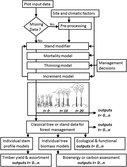
A flow chart representing the CARBWARE model inputs, functionality and outputs over time (t) for any given year (n). The model is initiated at time zero (t0). Diagram has been modified and adapted from Pretzsch et al. (2002).
Model simulation can be initiated with traditional single-tree mensuration data such as diameter at breast height (1.3 m, DBH), ideally for every tree within a user-defined plot area. Individual tree species should also be identified together with information on whether trees are alive or dead at the time of the inventory. A sub-sample of trees within the plot should be measured for tree height (H) and live crown ratio (CR).
The growth and mortality models have been developed for 12 common forest tree species growing in the Republic of Ireland. For the described species models presented in this paper, the application of the simulator is limited to trees with a minimum DBH of 7 cm.
The time step for the projection is 1 year, but it should be noted that the model was calibrated for trees measured over 4–6 year cycle.
Calibration data
Sample plot data
For this study, growth and mortality models were recalibrated using NFI data from the 2005/6 and 2010/12 inventories. Detailed methodologies used in the NFI can be obtained via a website link and Forest service publications (http://www.agriculture.gov.ie/media/migration/forestry/nationalforestinventory and Forest Service, 2007b).
A total of 16 280 repeat tree measurements over a period of 4–6 years were available, of which 8909 and 1951 measurements were taken from the Sitka spruce and Lodgepole pine strata, respectively (Table 1). Repeated measurements on trees from intimate mixed plantations of these species accounted for 6 and 14 per cent of the Sitka spruce and Lodgepole pine strata, respectively.
Details of tree and stand variables for species sampled from the NFI database
| Species common name | Lodgepole pine | Sitka spruce |
|---|---|---|
| Binomial name | Pinus contorta Loud. | Picea sitchensis (Bong.) Carr. |
| Number of tree measurements | 1951 | 8909 |
| DBH mean (cm) | 21 | 23 |
| Min | 7 | 7 |
| Max | 52 | 115 |
| BA mean (m2 ha−1) | 70 | 58 |
| Min | 3 | <1 |
| Max | 511 | 389 |
| CCF mean (%) | 385 | 328 |
| Min | 24 | 7 |
| Max | 1048 | 1655 |
CCF = crown competition factor; see equation 6.
where APlot is the plot total plot area and Ai denotes the area of the concentric circle associated with the ith diameter class.
Tree data with DBH, H and CR measurements were used to calibrate the H and CR models. The DBH increment models were calibrated using the repeated DBH measurements of trees taken over the two inventory cycles. Diameter increment was normalized to 1-year increments for model calibration.
Site and climatic factors
The NFI provides useful site information such as plot grid coordinates (in Irish national grid), soil type, elevation (E, in m) and slope (S, in per cent). An additional 50-m DEM was used to derive a topographical position index (TPI) based on the difference in the elevation value of a raster cell relative to neighbourhood cells (Black et al., 2014).
Climatic factors and other site factors, which are known to influence tree growth, were derived using the Irish ecological site classification system (ESC, Black et al., 2014; Ray et al., 2009). Accumulated temperature (range 1500–1850 day degrees, AT) above a threshold temperature is used as an ecological determinant of warmth. AT above 5°C was calculated using gridded daily values of maximum and minimum air temperature at a 50-m resolution (Black et al., 2014). Moisture deficit (range 0–189 mm, MD) is defined as the excess of rainfall over evaporation for the growing season (March–October), expressed as the cumulative difference between rainfall and evaporation. Wind exposure was expressed using the detailed aspect method of scoring (DAMS, Quine and White, 1994). Soil descriptions from the NFI PSPs were used to derive soil moisture regime (SMR) and soil nutrient regime (SNR, Pyatt et al., 2001). The ESC factor data are available for the island of Ireland in raster format (see http://82.165.27.141/climadapt_client/index.jsp).
Core models
Pre-processing
The representative tree number (EF) is only included (see equation 1) when all trees in the plot are not measured, as is the case for the random stratified sample used in the NFI.
Stand modifier
The stand modifier module (see Figure 1) updates individual tree DBH, H, BAL, cw and CR values for the initiation year (t0), based on simulated diameter and height increments for the current year (tn) before the next annual simulation is run (tn+1). Plot-specific variables such as BA and CCF are also modified. The software removes harvested trees from the input data files, as specified in the management decision module (See Figure 1), and stores these in a thinning or harvest table. If a tree has been predicted to have died, based on the mortality model threshold, it remains in the plot but does not undergo further increment computations.
Mortality models
A probability on the logit scale to the binary (dead, alive) scale was based on the observed overall mortality rates over a 36-year period. Models were optimized (maximum likelihood) using the highest goodness-of-fit and the calculated area under the receiver operating characteristic (ROC) curve (Heagerty et al., 2000). Here, correctly predicted tree mortality rate (i.e. a true-positive rate, TPR) is plotted against the false-positive mortality rate (FPR—the rate at which the model predicted mortality incorrectly) with the cut-off (P-value on the same Y-axis as TPR). The area under the ROC curve (AUC) is the estimated probability that the classifier will give a higher score to TPR cases than FPR cases. Specifically, a cut-off (P-value) was chosen to keep the rate of trees incorrectly predicted as dead (false-positive rate (FPR)) as small as possible, whilst ensuring that the overall mortality for the observed and predicted values was not due to chance (i.e. AUC > 0.5).
Thinning functionality
Harvesting of individual trees can be simulated using a range of potential selective thinning scenarios including: non-selective thinning and a range selective thinnings (i.e. tree number, BA, target diameter, stand density index, competition index). However, for the purposes of this study, non-selective thinning was carried out using a user-defined BA threshold (i.e. stems are randomly removed from a list, their EF is set to zero and the process is repeated until the BA threshold is met).
Growth increment models
Some ESC factors, such as DAMS, AT and MD, were excluded as model parameters because these did not improve model performance. Once Dinc has been simulated, the corresponding increase in tree height is estimated using equation 2. The outputs from the growth model are then either used to recalculate model parameters in the stand modifier module before the next annual time step simulation is initiated or to provide classical stand-based estimates (Figure 1).
Outputs
Stand management data
Once a time series has been simulated, individual tree data can be aggregated to the stand level to derive traditional metrics to aid in management decisions. These include BA, trees per hectare, mean DBH, DBH distribution, mean H, CCF and per cent mortality. These data can be queried from the database before the next management intervention selected (management decision module, Figure 1) and simulated.
Timber yield and assortment outputs
Generalized species-specific parameterizations of equations 17–19 were carried out by Dr M. Cerney (IFER, Czech Republic) using the non-linear least-squares method, based on 214 016 Sitka spruce and 94 601 Lodgepole pine stem profile data taken from the Coillte PSP database (Černý et al., unpublished data, but all parameters are shown in Supplementary data, Table S4A).
Individual stem diameters were derived at 0.5-m intervals using the stem profile model, and the volume of sections was estimated by applying a frustum of cone geometric equation (Matthews and Mackie, 2006). Total tree volume was simply derived as the sum of volumes for all 0.5-m sections. All volumes are based on a stump height at 1 per cent of total tree height.
Model selection and calibration
All models were calibrated using the NFI data for Sitka spruce and Lodgepole pine (Table 1). Selection, grouping and formulation of variables used in the models were initially based on formulations used by Monserud and Sterba (1996) with additional site, climatic and topographical variables added or removed in a step-wise manner using the R studio package MASS (Venables and Ripley, 2002). The procedure uses Akaike information criteria (AIC) for model selection in order to avoid over parameterization of the model (see Burnham and Anderson, 2002) based on the condition that the AIC values should decrease at each step.
Tree height model formulations published by Hawkins et al. (2012) were recalibrated using the NFI data and used as an internal benchmark (based on ΔAIC) to test whether model performance did improve when new formulations were used and site factors were included.
For the Dinc model calibration, the stepwise model selection was first done for individual sub-models (SITE, COMP, ESC and TOPO; see equations 11–15) using ΔAIC. In order to evaluate the proportion of variation in tree growth, as explained by factors, the individual contribution of the sub-models was assessed using the multiple coefficient of determination (R2) assuming that there are no inter-correlations between these main factors (Monserud and Sterba, 1996). Original model formulations published by Monserud and Sterba (1996) were recalibrated and used as an internalized benchmark (based on ΔAIC) to test whether model performance did improve when new formulations and site factors were included (equation 10).
Model performance
Goodness of fit of final calibrated models was assessed using root mean squared error (RMSE) and bias (van Laar and Akça, 2007). Regression analysis of predicted and observed values was performed together with a normality test on model residuals using the Shapiro–Wilk statistic in R studio. The frequency distribution was considered to be normally distributed if the P-value of the Shapiro–Wilk estimate was >0.05.
Analysis of variance (ANOVA) was also used to derive F-values, as measure of goodness of fit in terms of how well the predicted model estimates described the variation in observed data.
For the validation data set, where sample size was <30, the non-parametric Wilcoxon signed rank test was used to test for significant differences between the median of observed and predicted values. The median values were assumed to be significantly different when the P-value of the Z-score was <0.05.
Demonstration/validation plots
A series of thinning and mixed Sitka spruce/Lodgepole pine experimental trials were selected from the Coillte Teoranta's PSP data base (Table 2) to validate mortality and growth increment models. Experimental plots were initially designed for stand-level assessments of different silvicultural treatments. The database recorded basic individual tree metrics with derived variables (volume) and the condition of trees where assessed including mortality. For a detailed description of the database, refer to Broad and Lynch (2006a,,b) and Hawkins et al. (2012). The selected plots (Table 2) were the only available experimental plot series for validation because most of the PSP experimental series have no data on plot locations and soil information. ESC and topographical factors (TOPO) were derived for the selected plots with known site location data using raster data and GIS approaches described by Black et al. (2014).
Details of experimental plot series used for the validation of mortality, growth and volume yield models
| Series | |||
|---|---|---|---|
| MCM8080202-4 | BGN016601-3 | BGN0166014/19/23 | |
| Species | Sitka spruce/Lodgepole pine mix (50:50) | Sitka spruce | Sitka spruce |
| Treatment | Intimate mixed-species selective thinning | Pure species, no thin | Pure species, selective thinning |
| Soil | Blanket peat | Brown earth | Brown earth |
| Location | Knocknagappul, Co. Cork | Ballinglen, Co. Wicklow | Ballinglen, Co. Wicklow |
| Plant year | 1966 | 1966 | 1966 |
| Thin years | 1982, 1988 | none | 1988, 1997, 2002 |
| Years assessed | 1982, 1983, 1988 | 1983, 1988, 1996, 2006 | 1983, 1988, 1997, 2002, 2006 |
| No. of plots | 9 | 12 | 15 |
| No. of repeat measurements | 2 | 3 | 5 |
| DBH range (cm) | 7.7–24.8 | 9.3–52.1 | 8.4–57.8 |
The reported DBH range includes living trees only.
All selected plots were planted in 1966 at initial densities of 2500 trees per ha followed by a thin or no thin treatment. Models were initiated based on the first assessments of DBH and some H and CR measurements taken in 1982/3. For the thinning treatments (i.e. series BGN0166014/19/23 and MCM8080202-4, Table 2), the non-selective thinning option used by the CARBWARE model was not used. In this case, the same trees were removed from the tree tables as those removed from the experimental plots. Therefore, the thinning functionality of the simulator was not validated. The mortality functions were included in the validation using the cut-off values derived during the model calibration. Stand volume was estimated from modelled and corresponding measured tree data from each plot using the generalized taper equations (equation 16). Therefore, the validation does not test the performance of taper equations but rather demonstrates the use of taper equations in deriving stand volume.
The validation was intended as a sub-model validation of individual tree diameter increment and stand mortality only. Stand variables were used to demonstrate the application of the simulator for the most commonly required management outputs. Assessment of stand mortality and standing volume were based on all initial and repeated measures from plot data (i.e. 9 (3 measurements from 3 plots)) to 15 (5 measurements from 3 plots) depending on the experimental series (Table 2). The validation of stand current annual increment was only based on repeat plot measurements (i.e. n = 9–12 plots).
Results
Model calibration
Tree H and CR models
Model formulations for predicting individual tree height, as published by Hawkins et al. (2012), were re-calibrated using the NFI data and used as an internalized measure of the improvement to model performance by the introduction of site-specific factors. The redeveloped tree height models (equation 2) for Sitka spruce and Lodgepole pine out-performed the original model formulation published by Hawkins et al. (2012), in terms of a lower AIC value, a lower RMSE, bias values and a higher R2 and F-value (Table 3). Calibrated CR models did not perform as well as individual tree height models but showed no significant bias in the prediction of CR values (Table 3). The lower R2 and F-values for the CR model, compared with tree height models, suggest that the CR model explained less variation in measured CR.
Performance of tree height (H) and CR models for Sitka spruce and Lodgepole pine trees sampled in the 2006 and 2012 NFI
| H (Hawkins et al., 2012) | H (equation 2) | CR (equation 6) | |
|---|---|---|---|
| Sitka spruce | |||
| R2 | 0.88 | 0.91 | 0.64 |
| RMSE (cm) | 1.94 | 1.42 | 0.09 |
| Bias (cm) | −0.23 | 0.01 | <0.01 |
| F-value | 24 963 | 31 837 | 5181 |
| ΔAIC | 910 | ||
| N | 3745 | 3745 | 3722 |
| Lodgepole pine | |||
| R2 | 0.71 | 0.83 | 0.59 |
| RMSE (cm) | 1.98 | 1.72 | 0.11 |
| Bias (cm) | −0.22 | 0.02 | <0.01 |
| F-value | 2213 | 2442 | 1108 |
| ΔAIC | 326 | ||
| N | 904 | 904 | 902 |
The H model formulation published by Hawkins et al. (2012) was also re-calibrated using the NFI data for comparison. The regression and ANOVA test estimate of the F-value was significant at P < 0.01. A positive change in AIC (ΔAIC) indicates an improvement in the final H model (equation 2) over the formulation presented by Hawkins et al. (2012).
The models predict that variations in tree height and CR are influenced by site-specific factors (Supplementary data, Table S1A). For Sitka spruce, the model predicts that tree height generally decreases as elevation and TPI increases based on the negative value of the derived coefficients for these parameters (d3 and d5 in Supplementary data, Table S1A). For Lodgepole pine, exposure appears to have a larger influence on tree height, where the model predicts that height generally deceases with an increase in exposure (DAMS, d1Supplementary data, Table S1A). The CR of Sitka spruce trees appears to be influenced by elevation, with a decrease in live CR as elevation increases (d2, Supplementary data, Table S1A). The CR model for Lodgepole pine predicts that CR decreases as TPI values increase, suggesting a lower CR in sites located on ridges and hill tops (d3, Supplementary data, Table S1A).
Mortality models
Mortality rates for Lodgepole pine (5.6 per cent) over the 3- to 6-year period were higher, when compared with Sitka spruce (1.6 per cent), possibly due to the higher frequency of non-thinned stands and self-thinning, where northern provenances of Lodgepole pine are planted in mixtures with Sitka spruce. The Lodgepole pine sample contains a higher proportion of these types of stands, when compared with Sitka spruce.
All SITE factors were found not to significantly influence mortality in this study (Supplementary data, Table S2A). This may be due to the fact that one of the input variables is modelled Dinc, which already incorporates site variables in the growth model. The absence of a site effect may also be due to the small sample size of dead trees over the relatively short time period (3–6 years).
The final cut-off P-values were chosen by keeping the FPR as small as possible and by also ensuring that a similar mortality rate was obtained as the calibration data set. The AUC of plots shown in Figure 2 were 0.83 and 0.72 for Sitka spruce and Lodgepole pine, respectively, suggesting a reasonable fit (Supplementary data, Table S2A). However, there is still a trade-off between selecting a cut-off P-value where predicted mortality rates are similar to those in the observed data set, but without falsely predicting mortality of healthy trees. To illustrate this trade-off, the cut-off value for Sitka spruce was 0.15 when the overall predicted mortality rate was identical to the observed rate (1.6 per cent, see dotted line in Figure 2). However, at this cut-off value, only 36 per cent of the predictions were true-positive dead trees with 1.4 per cent being false-positive dead trees (Figure 2a). For Lodgepole pine, the optimized cut-off P-value is 0.23, which means that there is a higher prediction of the FPR (9.2 per cent), when compared with the Sitka spruce model (1.4 per cent, Figure 2).
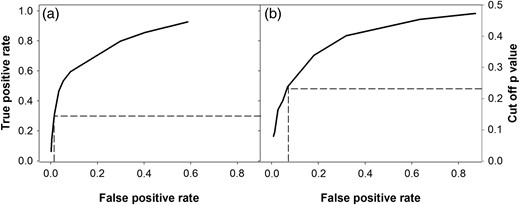
The influence of the cut-off P-value on the rate of predicting true-positive (observed mortality) and false-positive (mortality predictions for living trees) tree mortality in Sitka spruce (a) and Lodgepole pine (b). Note that the data presented for Sitka spruce and Lodgepole pine trees include the data taken from trees grown in mixed stands.
To ensure that the selected cut-off values did not result in a bias prediction of morality across the range of DBH and BAL values, histograms of observed and predicted mortality rates were compared (Figure 3). There was generally good agreement between observed and predicted mortality rates across the DBH and BAL ranges (Figure 3). Mortality of Lodgepole pine trees was, however, overestimated in the high BAL category (Figure 3). This issue could not be resolved by testing non-linear model formulations or by including additional variables into the model. The BAL category of 40+ m2 ha−1 is well represented in the calibration data set (21 per cent of all data for Lodgepole pine), but there was a proportionally higher (35 per cent) number of trees from mixed stands in this BAL category, compared with categories with low BAL values. When trees from mixed stands were excluded from the analysis, shown in Figure 3, the estimated mortality in the BAL 40+ category decreased from 18 to 11 per cent (data not shown). As expected, the mortality rate for species tested was higher in smaller trees (low DBH values) and/or where suppression was higher (i.e. at high BAL values, Figure 3). This is consistent with the negative slope for the fitted coefficient a3 and positive slope for coefficient a2 for Model 9 (see Supplementary data, Table S2A). There is also a large negative slope for the Dinc coefficient (a4, Supplementary data, Table S2A).
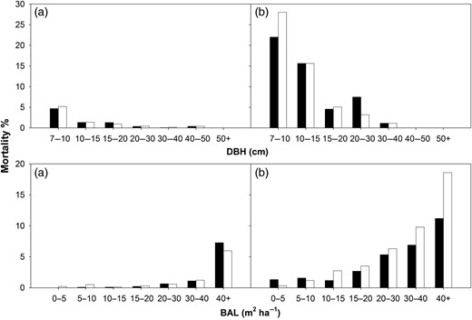
Observed (black histograms) and predicted (white histograms) mortality rates for Sitka spruce (a) and Lodgepole pine (b) across a range of DBH and BAL measurements. Note that the data presented for Sitka spruce and Lodgepole pine trees include data taken from trees grown in mixed stands.
Growth increment models
Diameter increment model selection was based on the initial inclusion of parameters for the SIZE sub-model (equation 11) followed by a stepwise inclusion of parameters for the other sub-models (COMP, ESC and TOPO) using AIC values as a guide. For Sitka spruce, inclusion of all sub-models resulted in an improvement to overall model performance (Table 4). However, the inclusion of parameters characterizing the influence of TOPO on the growth of Lodgepole pine did not improve model performance (Table 4).
The proportion of variation (R2, %) explained by major factors influencing the diameter increment (Dinc) model (equation 10) for Sitka spruce and Lodgepole pine
| Sub-model | Sitka spruce | Lodgepole pine | ||
|---|---|---|---|---|
| r2 | ΔAIC | r2 | ΔAIC | |
| SIZE (equation 11) | 17.2 | – | 19.7 | – |
| COMP (equation 12) | 22.1 | 492 | 29.5 | 546 |
| ESC (equation 14) | 8.9 | 80 | 3.9 | 36 |
| TOPO (equation 15) | 2.1 | 19 | n.s. | −2 |
| Sub-model | Sitka spruce | Lodgepole pine | ||
|---|---|---|---|---|
| r2 | ΔAIC | r2 | ΔAIC | |
| SIZE (equation 11) | 17.2 | – | 19.7 | – |
| COMP (equation 12) | 22.1 | 492 | 29.5 | 546 |
| ESC (equation 14) | 8.9 | 80 | 3.9 | 36 |
| TOPO (equation 15) | 2.1 | 19 | n.s. | −2 |
A positive change in the AIC value (ΔAIC) indicates a progressive improvement in model selection as sub-models are added to the final model formulation in a stepwise manner.
Final model formulations performed well, in terms of a low RMSE and no bias, across different stand types (Table 5). In addition, the final model formulations (Equations 10–15) performed better than those described by Monserud and Sterba (1996), based on an internalized comparison of AIC values (see ΔAIC, Table 5). The Dinc models described 50–53 per cent of the variation in diameter growth, based on the r2 from regression analysis of observed vs predicted Dinc values (top panel, Figure 4). Although the scatter plots of predicted vs model residual values may suggest a problem of heteroscedasticity, particularly for the Lodgepole pine model, subsequent Shapiro–Wilk tests confirmed that model residuals were normally distributed for both species (Figure 4). The F-value from ANOVA was significant for pure stands and for Sitka spruce and Lodgepole pine mixtures but was not significant for other mixed conifer and Sitka spruce stands (Table 5).
Growth model performance for Sitka spruce and Lodgepole pine across different forest categories (pure, or mixed conifer stands)
| Pure plantation | Lodgepole pine/spruce mixtures | Other conifer mixtures | All combined | |
|---|---|---|---|---|
| Sitka spruce | ||||
| RMSE (cm) | 0.211 | 0.26 | 0.395 | 0.237 |
| Bias (cm) | <0.001 | 0.005 | 0.044 | 0.003 |
| F-value | 3725.91 | 8.28 | 0.94 | 3882.45 |
| ΔAIC | 214 | |||
| N | 8374 | 354 | 181 | 8909 |
| Lodgepole pine | ||||
| RMSE (cm) | 0.175 | 0.298 | NA | 0.198 |
| Bias (cm) | <0.001 | 0.023 | NA | <0.001 |
| F-value | 689.22 | 57.13 | NA | 700.39 |
| ΔAIC | 245 | |||
| N | 1677 | 247 | NA | 1951 |
The regression and ANOVA test estimate of the F-value was significant at P < 0.01. A positive change in AIC indicates an improvement in the performance of the final model (equation 10) over the formulation presented by Monserud and Sterba (1996).
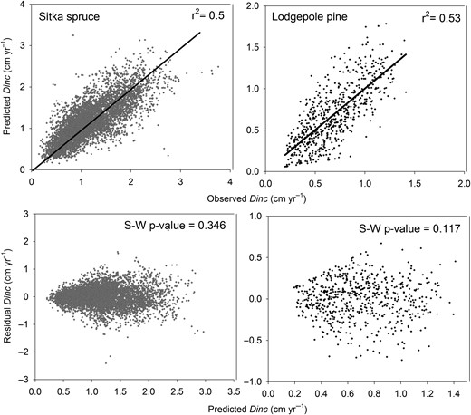
Regression analysis of predicted vs observed (top panel) and model residuals vs predicted Dinc values (bottom panel) for Sitka spruce (grey symbols, n = 8909) and Lodgepole pine (black symbols, n = 1951). The solid regression line represents a significant r2 at P < 0.05. The P-value of Sharipro–Wilk statistic (S–W P-value) confirmed a normal distribution of model residuals at P < 0.05. Note that the data presented for Sitka spruce and Lodgepole pine trees include NFI data taken from trees grown in mixed and pure stands.
Growth variables for competition (COMP) factors in equation 12 described most of the variation (22–29 per cent) in tree growth (Dinc) for both species tested (Table 4). In all cases, growth increment significantly decreased as BAL increased, as evident from the negative slope of the coefficient b2 in equation 12 (Figure 5, Supplementary data, Table S3A). This is expected since growth of non-dominant trees would decrease as competition in the stand increases. The higher negative slope for coefficient b2 (see Supplementary data, Table S3A) for the Lodgepole pine, compared with the Sitka spruce model, suggests a higher reduction in individual growth as BAL increases.

Observed (black histograms) and predicted (white histograms) diameter increment (Dinc) for Sitka spruce (a) and Lodgepole pine (b) across a range of BAL and CCF values. Note that the data presented for Sitka spruce and Lodgepole pine trees include data taken from trees grown in mixed stands.
CCF was also a significant COMP factor influencing tree growth (see coefficient b3Supplementary data, Table S3A, Figure 5). Again, the higher negative slope of coefficient b3 for Lodgepole pine suggests a greater reduction in individual tree growth as available light in the canopy decreases.
Tree SIZE factors explained 17.2–19.7 per cent of the observed variation in tree growth (Table 4). CR is a simple measure of potential capacity to capture light and appeared to be the most important SIZE factor influencing tree growth. This is based on a higher slope for the coefficient a4, when compared with DBH-derived coefficients (Supplementary data, Table S3A and Figure 6) and the largest ΔAIC value when CR was included in the SIZE sub-model (data not shown). The slope for coefficient a4 in equation 12 was higher for Lodgepole pine, when compared with Sitka spruce (Supplementary data, Table S3A).The Ln(DBH) was significant predictor of growth for both species and showed an increase in vigour for larger DBH trees (Figure 6, Supplementary data, Table S3A). The parameter DBH2 effectively reduces the increase in tree growth as DBH increases, but this was only significant for Sitka spruce (Supplementary data, Table S3A).
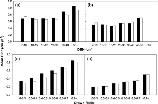
Observed (black histograms) and predicted (white histograms) diameter increment (Dinc) for Sitka spruce (a) and Lodgepole pine (b) across range of DBH and CR values.
SITE factors explained 3–11 per cent of the variation in tree growth (Table 4). ESC factors accounted to most of the site-specific variation in tree growth. Most notable were SNR and SMR, which influenced tree growth for Sitka spruce (coefficients c2 and c3 in Supplementary data, Table S3A). The positive slope of coefficients c2 and c3 indicates that vigour of Sitka spruce increases in more fertile and on drier/drained soils (Supplementary data, Table S3A, Figure 7). SNR was the only significant ESC factor influencing growth of Lodgepole pine. Other climatic factors such as AT and MD appeared to have no significant effect on tree growth. Inclusion of climatic variables during model selection resulted in no change or an increase in the AIC value for the SITE sub-model. It is important to note that there is a small climatic gradient across the Republic of Ireland. For example, over 90 per cent of the total area falls within the warm moist climatic zone (AT and MD classified zones in ESC (Pyatt et al., 2001)). The warm wet climatic zones are confined to 5 per cent of the land area, mainly in the west of Kerry, parts of Connemara and northern Donegal. Only 4 per cent of the land area in south Wexford falls in the warm dry zone. In contrast, the UK is represented by seven climatic zones varying from alpine to warm dry zones (Pyatt et al., 2001).
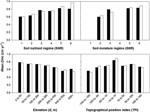
Effect of SITE factors on observed (black histograms) and predicted (white histograms) diameter increment (Dinc) for Sitka spruce.
TOPO only accounted for 2.1 per cent of the variation in growth of Sitka spruce. In this case, the effect of TPI was quadratic (see equation 15). TPI values varied from −135 to 125 (Figure 7). Negative values indicate valley bottoms or depressions and positive values represent hilltops or ridge tops. The derived coefficient d3 (Supplementary data, Table S3A) was close to zero for Sitka spruce, and the optimal topographical position for growth appears to be on flat or mid slope areas (Figure 7). The effect of elevation (E) on growth was linear for Sitka spruce with a decreasing trend in growth as E increased (i.e. negative slope for coefficient d4, Supplementary data, Table S3A).
Independent validation and demonstration of model application
The stand simulator provided reasonable estimates of derived stand volume and current annual increments over a 50-year rotation for different thinning regimes and intimate mixtures (Table 6). All of the available Coillte PSP data for intimate Lodgepole pine and Sitka spruce mixtures had limited repeat measurements. Therefore, it was not possible to evaluate the mortality and growth model performance for intimate mixtures at ages close to rotation age. There was no significant difference (P > 0.05) in the mean (F-value) or median (Wilcoxon signed rank) for observed and predicted estimates of individual tree growth and stand volume across all silvicultural regimes tested (Table 6). The stand simulator also provided a good estimate of stand mortality for no thin and thinned Sitka spruce experimental plots (Table 6) and correctly predicted a higher mortality rate (a 6 per cent increase) for no thin stands as expected. The F-value for estimated stand mortality rates in intimate mixed Lodgepole pine and Sitka spruce plots was not significant, suggesting that the model did not explain the variation in observed mortality in these plots. Although there was an overestimation of mean stand mortality by 2.3 per cent, the Wilcoxon signed rank test suggests that this was not significant. The use of non-parametric Wilcoxon signed rank test may be a more suitable statistical procedure for small sample sizes, as was the case for this experimental series, but the small sample size of the validation set is a confounding factor when interpreting these results.
Growth model performance for pure and mixed Sitka spruce and Lodgepole pine across three commonly used silvicultural regimes in the Republic of Ireland
| Dinc (cm year−1) | Standing volume (m3 ha−1) | Volume increment (m3 ha−1 year−1) | Mortality rate (mean %) | |
|---|---|---|---|---|
| Sitka spruce thin (series BGN0166014/19/23) | ||||
| RMSE | 0.18 | 22.4 | 2.7 | 1.2 |
| Bias | 0.014 | 3.03 | −0.7 | 0.3 |
| WC P-value | 0.66 | 0.51 | 0.46 | |
| F-value | 498.41** | 114.85** | 75.99** | 24.63* |
| S–W P-value | 0.94 | 0.32 | 0.10 | 0.21 |
| N | 621 | 15 | 12 | 15 |
| Sitka spruce no thin (series BGN0166001-3) | ||||
| RMSE | 0.19 | 47.1 | 3.1 | 5.3 |
| Bias | −0.021 | −7.6 | 0.5 | 0.7 |
| WC P-value | 0.81 | 0.92 | 0.3 | 0.21 |
| F-value | 547.36** | 169.34** | 87.79** | 10.05* |
| S–W P-value | 0.81 | 0.29 | 0.14 | 0.21 |
| N | 851 | 12 | 9 | 12 |
| Sitka spruce/Lodgepole pine (series MCM8080202/3) | ||||
| RMSE | 0.23 | 30.4 | 1.3 | 4.1 |
| Bias | −0.07 | −12.1 | −0.3 | 2.8 |
| WC P-value | 0.38 | 0.21 | 0.08 | |
| F-value | 389.91** | 25.74* | 15.34* | 0.47 |
| S–W P-value | 0.52 | 0.25 | 0.31 | 0.14 |
| N | 394 | 9 | 6 | 9 |
There was no significant difference between the observed and predicted estimates when the Wilcoxon (WC) P-value is >0.05. The regression and ANOVA test estimate of the F-value was significant at P < 0.05* and P < 0.01**. The model residual values are assumed to be normally distributed if the P-value of Shapiro–Wilk (S–W) test is >0.05. Refer to Table 2 for details of selected experimental plot series.
Analysis of model residuals using Shapiro–Wilk statistics for individual tree Dinc, stand volume, annual volume increment and per cent mortality suggests that estimated model residual values are normally distributed (Table 6). However, caution should be applied when interpreting the Shapiro–Wilk test for small sample sizes.
Discussion
This paper describes the growth and mortality models underlying the CARBWARE stand simulator. The distance-independent single-tree growth modelling framework described by Wykoff (1990) and Monserud and Sterba (1996) has been modified to include spatially explicit ESC system climatic and soil factors, for application to Irish and UK forestry. The ESC system developed for Ireland (Ray et al., 2009) and the UK (Pyatt et al., 2001) is based on a ‘Delphi’ calibration with no consideration of empirically based observations on how climatic factors may influence site productivity. The results from this study suggest that AT of >5°C and MD have no significant site influence on single-tree growth of the major coniferous species grown in the Republic of Ireland. The absence of any apparent climatic influence on growth in this study may be due to numerous factors. For instance, most tree species occurring in Ireland, with the exception of Arbutus, do not occur at the extreme of their climatic range and, therefore, may not exhibit any significant response to variations in site temperature or MD. Secondly, the spatial or temporal scales at which climatic variables are measured, or downscaled to, may not be reflective of the site micro-climatic conditions (see Black et al., 2014). Thirdly, the NFI calibration data used in this study were collected over a relatively short time period (5 years). The use of long-term PSP data may provide a better insight into how climatic factors may influence growth or mortality, but only if site climate records or geo-referenced locations of sites are documented. Finally, the formulation and abstraction of the PROGNOSIS modelling framework may not adequately describe climatic responses to tree growth. This is because growth responses may show different dose effects to particular environmental factors, which are defined by the ecologically optimum or sub-optimum requirements to the limiting factor by the species of interest (see dose effect rule, Pretzsch, 2009). In other words, variations in growth due to a change in response to a climatic factor are proportional to the difference between the maximum and actual growth. The key issue is that the PROGNOSIS approach does not use differential equations where maximum growth is defined. Alternative models such as the potential modifier method, dose–response functions, gap models or hybrid-process-based approaches (see Pretzsch, 2009) may provide a more effective way of characterizing growth responses to the climatic factors. Such models may, therefore, be more useful for functional and ecological analysis, such as the influence of future climate change on tree growth.
The calibrated models for Sitka spruce and Lodgepole pine describe an overall variation of 50–53 per cent in single-tree growth, which is comparable with other PROGNOSIS model applications in the USA and Austria (25–68 per cent, see Wykoff, 1990; Monserud and Sterba, 1996). These authors suggest that tree size factors describe most of the variation in tree growth (20–44 per cent) for species occurring in those regions, followed by competition factors, which only described 7–15 per cent in single-tree diameter increment. In contrast, competition appears to be the most important factor influencing diameter increment for both species investigated in this study, describing 22–30 per cent of the variation (Table 4). The greater influence of competition factors on tree growth, in Ireland, compared with other regions may not be surprising given the higher crown cover intensity of plantation forestry and the greater potential for growth suppression by a typical closed canopy conifer stand. For example, the maximum reported CCF for conifer stands in Austria is 699 (Thurnher et al., 2011), compared with over 1600 for Sitka spruce stands in Ireland (Table 1). The greater suppression of growth in Irish conifer stands is illustrated by the 6- to 10-fold higher negative slope of the competition factor coefficients BAL and CCF (Supplementary data, Table S3A), when compared with conifer stands in Austria (Monserud and Sterba, 1996). Given the apparent importance of these competition factors on tree growth, further modelling improvements may be possible by deriving region specific open-grown crown width (cw) models. Currently used models (see equation 4) are based on data derived for similar species in Austrian forests. Site factors only explained 3–11 per cent of the variation in tree growth (Table 4). Monserud and Sterba (1996) reported that site factors (topography only) described a 2–6 per cent of the variation in tree growth. Differences between these reported estimates may be indicative that the additional influence of ESC factors could explain some of the variation in single-tree growth and these may be useful site variables to include in the PROGNOSIS model framework. The only significant ESC factors influencing single-tree growth for species investigated were SNR and SMR (equation 14, Supplementary data, Table S3A). This is consistent with a related site classification publication by Farrelly et al. (2011), who show that SNR and SMR explained 51 per cent of the variation in the site index of Sitka spruce. However, our results suggest that these ESC factors only explain 3–9 per cent of the site to site variation in growth. TOPO only explained 2 per cent of the site to site variation in growth of Sitka spruce. This is surprising since elevation, aspect and TOPEX have been suggested to influence growth of conifer species in Ireland (Horgan et al., 2004). Although TOPEX was not used in this study, TPI was used instead because it is a more easily derived surrogate measure of exposure and shelter, based on digital elevation models (Black et al., 2014). The growth response to variations in TPI suggests that the highest growth rates for Sitka spruce occur a low to zero TPI scores (Figure 6), which are indicative of valley bottoms or sheltered mid slopes. Monserud and Sterba (1996) reported a significant reduction in growth of Norway spruce on north-facing slopes in Austria. This was not evident in this study, even though Sitka spruce has been suggested to be less suited to northern-facing slopes (Horgan et al., 2004).
Species comparison of growth responses to competition and site factors may provide some insight into the physiological characteristics of the species in relation performance under current silvicultural practice. For example, the magnitude of the slope (i.e. coefficients b2 and b3, Supplementary data, Table S3A) of growth responses to competition factors was consistently higher for Lodgepole pine, when compared with Sitka spruce. This suggests that the growth of Lodgepole pine may be more sensitive to crown competition than Sitka spruce. This would be consistent with the idea that Lodgepole pine is a light-demanding species, compared with a Sitka spruce, which is an intermediate shade bearer (Horgan et al., 2004). Moreover, the higher mortality of Lodgepole pine in response to an increase in competition (BAL) and as growth rates decreases (Supplementary data, Table S2A, Figure 3) may suggest that this species may exhibit a higher degree of self-thinning, when compared with Sitka spruce. Different species responses to other edaphic factors are also evident. The lower sensitivity of Lodgepole pine to SNR (i.e. a lower value for coefficient c2, Supplementary data, Table S3A), compared with that for Sitka spruce, is also consistent with the lower nutrient requirement of Lodgepole pine (Horgan et al., 2004). The improved growth response of Sitka spruce in sheltered and low elevation sites is consistent with the natural distribution of the species in the coastal north-western pacific regions. In contrast, the absence of any significant influence of TOPO on growth of Lodgepole pine may reflect the suitability of the species at in more elevated sites and exposed sites. These findings may provide some empirical basis for potential improvement to current used Delphi-based ESC systems.
The independent stand-level validation of the growth simulator produced reasonable results with no significant bias in the estimation of stand volume or volume increment across the different species and silvicultural treatments (Table 6, Figure 7). These results are comparable to standing volume and volume increment estimates derived from other single-tree-based stand simulators, such as SILVA (Pretzsch et al., 2002, see Table 2 of their publication), who report a bias and precision of −1.9 per cent and 19.84 per cent, respectively, for an analysis done on 220 Norway spruce stands. Although the number of stands used in this study for validation was considerably lower, the corresponding bias and precision values of the pure Sitka spruce stands (n = 24) were −0.9 per cent and 11.24 per cent, respectively. It is difficult to compare the presented single-tree growth stand simulator with conventional stand-based models, such GROWFOR (Broad and Lynch, 2006b). However, Broad and Lynch (2006b) reported a bias of −0.37–2.33 per cent for standing volume from 1244 Sitka spruce plot observations and an adjusted r2 of 0.96. The adjusted r2 for validated stand volume for Sitka spruce stands investigated in this study is 0.98. Broad and Lynch did not, however, report on the precision of dynamic stand models for Sitka spruce. A high level of precision is an important requirement for management, planning and resource evaluation at the stand level. Nieuwenhuis et al. (1999) argue that accurate stand timber evaluation requires measured distributions of diameter distributions. Single-tree-based stand simulators offer this functionality.
One of the potentially uncharacterized variations in single-tree growth for the two species investigated in this study and in other similar studies (Monserud and Sterba, 1996; Hasenauer, 2006) is potential genetic differences within a given species. In Ireland, there has been a changing trend towards the establishment of more southern provenances of Sitka spruce, such as Washington and Oregon sources, replacing QCI (Thompson et al., 2005). More recently, improved clonal Washington material from the Irish Sitka breeding programme has been introduced into the estate (Lee et al., 2013). Results from IUFRO provenance trails and more recent progeny test trials suggest that different seed sources of Sitka spruce may result in a 2–4 yield class difference in productivity (Thompson et al., 2005; Lee et al., 2013). Based on the mean yield class for Sitka spruce in Ireland (ca. 18 m3 ha−1 year−1), this represents a potential genetic variation in productivity of 11–22 per cent. Similarly, various sources of Lodgepole pine have been introduced into Ireland, from inland, northern coastal to southern coastal provenances of the pacific north-west. However, no records are available from the NFI or Coillte inventory databases to distinguish provenance of a species for a given site. Although the precise variation in growth associated with inter-species provenance and genetic variation is difficult to estimate, indications are that this could be as high as 20 per cent. Clearly, provenance information should be included in single-tree model simulations, so that different models for different provenances of the same species can be developed. Empirical observations from such studies would also aid in the development of more precise ESC suitability decision support systems. The advantage of site index-based stand models is that genetic variation can be accounted for once potential yield class or sand index has been derived. Other single-tree modelling approaches such as the potential modifier method may also better characterize these genetic variations in growth (see Pretzsch, 2009).
The derived mortality rate responses to tree size, competition and vigour (see Figure 3 and Supplementary data, Table S2A) for both species suggest that mortality may increase as vigour declines in larger older trees or when competition from surrounding trees increase. Therefore, the DBH–mortality curve (Figure 3) may be expected to be U-shaped as the probability of mortality increased in less vigorous older trees. However, a very large sample of may be required to detect this in a normal forest inventory. The selected cut-off P-value for the two species may result in a low detection of true-positive dead trees (varying from 35 to 42 per cent) at the expense of incorrectly classifying living trees as dead trees. For comparison, a similar study conducted by Monserud and Sterba (1999) developed mortality models, which correctly predicted mortality in 25–46 per cent of dead trees. It is not clear why mortality for Lodgepole pine is overestimated at high BAL values (Figure 3). This may be associated with poorer model performance for mixed stands since a high proportion of trees in the 40+ m2 ha−1 BAL category come from mixed stands. This suggests that alternative model formulations, which quantify the effect of mixed-species interactions on mortality, may be required in the future. Although methods to quantify mixture effects at the individual tree level have been developed in terms of productivity efficiency (see Pretzsch, 2009), these have not been developed for mortality models. Another possible reason for the observed overestimation of mortality for Lodgepole pine at the larger BAL value categories is the complication of using NFI data for model calibration.
In conclusion, the described CARBWARE single-tree stand simulator provides a robust and un-bias estimate of single-tree and stand-based variables, which are comparable to other modelling approaches used in Europe. Although, the calibration, validation and demonstration of the model are the main focus of the paper, the simulator has numerous applications and advantages over traditional stand-based models. The simulator is currently used for national carbon reporting to the UNFCCC (Duffy et al., 2013) and has application potential for bucking optimization procedures to aggregate individual tree sections into user-defined assortment classes and log lengths (Nieuwenhuis et al., 1999). However, refinement of the models is still required, particularly improvement to climatic and genetic response factors, mortality functions for mixed-species stands, regeneration models and derivation of regional and species-specific crown structure algorithms. The lack of recruitment/regeneration models in the current CARBWARE simulator means that application should be limited to plantation forestry where natural regeneration or forest succession does not occur.
Conflict of interest statement
None declared.
Funding
This work was funded by the Council for Forest Research and Development (COFORD), Department of Agriculture, Food and the Marine under the Irish National Development Plan 2007–2013 [BetterFor project, ref 13 C451].
Acknowledgements
The author thanks John Redmond from the Forest Service, Department of Agriculture, Food and the Marine for the provision of NFI data. The Coillte PSP data were supplied by Ted Lynch. The author is also grateful to Duncan Ray, NRS Forest Research U.K. for provision of the ESC factor raster data. He acknowledges Michael Hawkins for his work on the development of earlier versions of the CARBWARE model, Mark Tarleton and Jacques Hamel for developing the software. He also acknowledges the significant contribution made by the review editor and reviewer.
References
